spatialkit

Spatial tessellation, modeling, and cross-validation toolkit for R

Contents

• The problem this solves
• Scope
• Installation
• Quick start
• Which function do I want?
• Choosing a backend
• Documentation
• Troubleshooting
• Running it in practice
• Development
• Project

The problem this solves

You have observations at points and you need values over areas. The path of least resistance is to borrow boundaries that already exist: ZIP codes, census tracts, counties, sales territories. Each was drawn for mail routing, enumeration or politics, and none of them knows anything about the process you are studying. Aggregate onto them and part of your answer is an artefact of the partition. This is the modifiable areal unit problem, and it is not a rounding error: the same observations can support materially different conclusions under different boundaries.

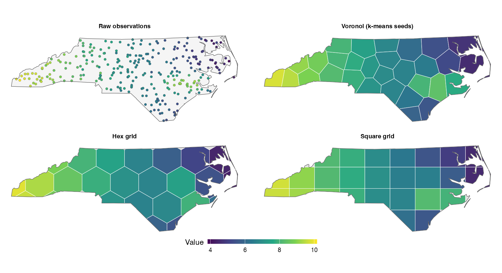
spatialkit lets the data draw the boundaries. get_voronoi_seeds() places seeds by k-means on the point cloud, so cell density follows sampling density. resolution_profile() scores every candidate cell count against the spatial structure of the observations, and determine_optimal_levels() reads one off their clustering when they have any. build_tessellation() produces Voronoi, hex, square or Delaunay cells clipped to your study area, with IDs that stay stable when the input row order changes. summarize_by_cell() aggregates onto them with a count and a standard error for every cell mean. When the cell means stand in for a population mean, it corrects those standard errors for within-cell autocorrelation, which on a correlated field can double them or more.

Redrawing boundaries is easy. Knowing whether the result means anything is the hard part, so the second half of the package is the evidence layer. Three model backends sit behind one spatial_fit class so they can be scored on identical folds. Cross-validation holds out whole regions sized to the data’s own autocorrelation range. An area-of-applicability estimate marks where the resulting score applies. All of it is built on sf, with CRS handling that will not hand metres to a function expecting degrees.

Raw spatial field and three tessellation methods aggregating it over North Carolina

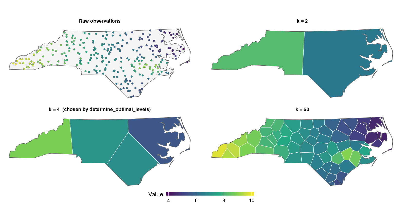
How many cells is a decision with visible consequences. The same field below is cut at three resolutions beside the raw observations: too coarse blurs the hotspot, too fine chases noise with near-empty cells, and the middle count, the one resolution_profile() rates most reliable, keeps the trend without tracing the sampling pattern. It is a reading, not a verdict: the reliability of the cell means stays within 2 percent of its best from 3 to 25 cells here, and the sites are spread evenly, so there is no elbow for determine_optimal_levels() to find. vignette("resolution") covers how that number is chosen and the four criteria that disagree about it.

Raw observations and the same spatial field tessellated at three resolutions, including the count resolution_profile() rates most reliable

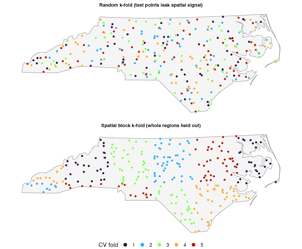
The number a random fold reports on autocorrelated data is the reason the evidence layer exists. Random folds put a test point’s neighbours in the training set, so a model with any capacity to memorise location already has the answer in front of it:

Random k-fold versus spatial block k-fold assignments across North Carolina

Scope

Everything above is what the package is for. Here is where it stops, so you can rule it out before spending time on the quick start:

• Regression only. A non-numeric response is refused outright, and an integer-coded binary response is refused by fit_gwr_model() with a pointer to GWmodel::ggwr.basic(). (A two-valued non-integer response, such as a measurement censored at a detection limit, is continuous, so it is fitted with a warning.) There is no classification path.
• Vector point data only. No raster support. predict_surface() returns an sf POINT layer; convert it downstream if you need a SpatRaster.
• No areal / lattice models. Moran’s I here is a residual diagnostic on point data. There is no CAR, SAR or spatial-lag fitter.
• No spatio-temporal folds. Every fold scheme is purely spatial.

Installation

# install.packages("remotes")
remotes::install_github("elkronos/gis_modeling_toolkit")

# with the vignettes (needs pandoc)
remotes::install_github("elkronos/gis_modeling_toolkit", build_vignettes = TRUE)

sf, dplyr, logger and digest install with it. Everything below is optional and needed only for the feature that uses it. A missing one produces a message naming it.

install	for
gstat	variogram fitting: estimate_sac_range(), design effects, kriging checks
ranger	fit_rf_model(), cv_rf()
sp, GWmodel	fit_gwr_model(), cv_gwr()
brms (plus a Stan toolchain)	fit_bayesian_spatial_model(), cv_bayes()
geometry	Delaunay triangle tessellations
ggplot2	every plot_*() function and plot() method
patchwork	the combined panels in vignette("spatialkit_nc_demo") and its script
FNN, Matrix	sparse k-nearest-neighbour weights for Moran’s I on large layers
loo	PSIS-LOO for the Bayesian backend
nlme	REML detrending in estimate_sac_range()
spdep	cross-checks in the test suite only

Quick start

Everything here runs on the hard dependencies alone. The learner is one lm() call wired in through new_spatial_fit(), so the whole arc executes without any optional backend.

library(sf)
library(spatialkit)

set.seed(42)
n  <- 400
xy <- data.frame(x = 5e5 + runif(n, 0, 1000), y = 5e6 + runif(n, 0, 1000))
D  <- as.matrix(dist(xy))
xy$w <- rnorm(n)
# Mostly a smooth spatial field, with a weak measured predictor on top.
xy$z <- 0.5 * xy$w +
  as.numeric(t(chol(exp(-D / 80) + diag(1e-8, n))) %*% rnorm(n)) +
  rnorm(n, sd = 0.3)
site <- st_as_sf(xy, coords = c("x", "y"), crs = 32632)

Draw regions from the data and aggregate onto them:

tess  <- build_tessellation(site, boundary = clip_target_for(site, quiet = TRUE),
                            method = "hex", approx_n_cells = 24, quiet = TRUE)
asg   <- assign_features_to_polygons(site, tess$cells)
cells <- summarize_by_cell(asg, "z", cells_sf = tess$cells, deff = "kish")

populated <- st_drop_geometry(cells)[cells$n > 1 & !is.na(cells$n), ]
head(populated[, c("poly_id", "n", "resp_mean_z", "..se_resp_z")], 4)
#>   poly_id  n resp_mean_z ..se_resp_z
#> 2       2 12  -0.3553720   0.3840250
#> 3       3  6  -0.7977035   0.6491918
#> 4       4  2  -1.8546732   0.1801251
#> 5       5 14   0.0554452   0.7258217

Every aggregate arrives with a count and a standard error. deff = "kish" makes that the standard error of each cell mean as an estimate of the population mean, widened by the design effect of the within-cell correlation. For a map of the cells’ own values leave deff at 1: the uncorrected standard error is the right one for a cell’s own mean when its points are spread through it (?summarize_by_cell says which to use when). A lattice laid over an irregular point cloud leaves some cells with one observation or none, which is why n travels with every row.

Now score a model. The learner below is a cubic trend surface in the coordinates, which is a realistic thing to fit and also the leakage mechanism this package warns about: given x and y, a flexible model can reproduce the training surface by memorising location.

trend_fit <- function(train_sf, ...) {
  d <- st_drop_geometry(train_sf)
  d$x <- st_coordinates(train_sf)[, 1]
  d$y <- st_coordinates(train_sf)[, 2]
  new_spatial_fit("trend_fit", engine = lm(z ~ w + poly(x, 3) * poly(y, 3), data = d),
                  formula = z ~ w + poly(x, 3) * poly(y, 3), response_var = "z",
                  predictor_vars = "w", data_sf = train_sf)
}
predict.trend_fit <- function(object, newdata = NULL, ...) {
  if (is.null(newdata)) return(fitted(object$engine))
  d <- st_drop_geometry(newdata)
  d$x <- st_coordinates(newdata)[, 1]
  d$y <- st_coordinates(newdata)[, 2]
  as.numeric(predict(object$engine, newdata = d))
}
residuals.trend_fit <- function(object, ...) residuals(object$engine)
fitted.trend_fit    <- function(object, ...) fitted(object$engine)
for (g in c("predict", "residuals", "fitted"))
  registerS3method(g, "trend_fit", get(paste0(g, ".trend_fit")))

# The blocks are sized to the field's own correlation: its effective range is
# 3 x 80 = 240 units, so 250-unit blocks hold out whole patches.  On real data
# the range is estimated, by estimate_sac_range() or make_folds(auto_range =
# TRUE); vignette("spatial-cross-validation") is about that choice.
random  <- cv_spatial(site, "z", "w", fit_fn = trend_fit,
                      folds = make_folds(site, k = 5, method = "random_kfold", seed = 1))
blocked <- cv_spatial(site, "z", "w", fit_fn = trend_fit,
                      folds = make_folds(site, k = 5, method = "block_kfold",
                                         block_size = 250, seed = 1))

c(random  = random$overall$RMSE,
  blocked = blocked$overall$RMSE,
  ratio   = blocked$overall$RMSE / random$overall$RMSE)
#>   random  blocked    ratio 
#> 1.011489 1.584805 1.566804

Same 400 observations, same model, one number more than half again the other. The difference is entirely in which rows were allowed to train on which, and the blocked figure is the one that answers the question a map is used for: what happens where there is no observation nearby.

Is there structure the model missed?

residual_morans_i(trend_fit(site))
#> Residual Moran's I = 0.3314   (E[I] = -0.0025, sd = 0.0236)
#>   z = 14.136, p = 2.275e-45
#>   null: randomisation moments, approximate for these residuals; n = 400, df = 399
#>   residual kurtosis 3.502 (3 = Gaussian)
#>   weights: 400 x 400 dgCMatrix, 8 neighbour(s) per row; not retained, keep_weights = TRUE to keep it

A large positive Moran’s I says the residuals of nearby points resemble each other, so something varying smoothly across the map is still missing. Note which null it used: the fit is not ordinary least squares on the declared predictor, so the exact residual moments do not apply and it fell back to the randomisation null, reporting itself as approximate.

Which function do I want?

I want to…	Use
get my data into a projected CRS	ensure_projected(), coerce_to_points(), harmonize_crs()
cut my study area into cells	build_tessellation() ("voronoi", "hex", "square", "triangles")
place the seeds a Voronoi grows from	get_voronoi_seeds()
choose how many cells, quickly (coordinates only, no optional packages)	determine_optimal_levels()
see what every cell count costs	resolution_profile(), then summary() on it for every criterion’s pick, or select_resolution() for one
put points into cells and aggregate	assign_features_to_polygons() → summarize_by_cell()
check whether a cell mean is the best estimate of that cell	kriging_adequacy()
draw the result	plot_tessellation_map()
know how far spatial correlation reaches	estimate_sac_range(), and sac_nugget() for its nugget
build honest CV folds	make_folds() (random_kfold, block_kfold, buffered_loo, leave_location_out, nndm)
see whether my folds actually separate	plot_folds()
size the blocks by measurement	cv_block_size_sweep(), and plot() on the result
fit a model	fit_gwr_model(), fit_bayesian_spatial_model(), fit_rf_model()
score it out of sample	cv_gwr(), cv_bayes(), cv_rf()
score my own learner on the same folds	cv_spatial() + new_spatial_fit()
score it in sample	model_metrics(), evaluate_insample(), compare_models()
see the fold-to-fold spread of a CV score	plot_cv_metrics()
check whether predicted intervals are the width they claim	plot_calibration()
pick predictors without leaking	select_features_forward() (gwr_model_selection() for the AICc counterpart)
compare backends head to head	compare_models_cv()
check for leftover spatial structure	residual_morans_i(), plot(fit, type = "variogram")
turn a fit into a map	predict_surface()
know where that map is extrapolation	area_of_applicability()
free memory held by the caches	clear_grid_cache(), clear_fitted_cache()

Lower-level exports sit behind these and have pages of their own: create_voronoi_polygons(), create_grid_polygons(), create_grid_polygons_cached(), clip_target_for(), ensure_stable_poly_id(), voronoi_seeds_kmeans(), voronoi_seeds_random(), prep_model_data() and gp_lengthscale_bounds(). The reference index lists everything, grouped by pipeline step.

Choosing a backend

compare_models_cv() scores all three on identical folds and is the right answer when you can afford it. It is not always cheap. On one recorded run (one machine, 4-fold CV, 2 chains × 1,000 iterations) the Bayesian GP took 1,186 s at n = 2,000 against 109 s for cv_gwr() on the same data. At n = 300 it was 142 s against 0.8 s, so the ratio is not fixed either. A cv_rf() of the same shape is seconds. So it is worth knowing what each backend is for before you spend an afternoon comparing them:

Backend	Reach for it when you want	Cost
GWR (fit_gwr_model(), GWmodel + sp)	spatially varying coefficients you can interpret and map. Only this backend answers “the elevation effect is strong in the west and absent in the east”	moderate; grows quickly with n
Bayesian spatial GP (fit_bayesian_spatial_model(), brms)	calibrated uncertainty: posterior predictive intervals, se = TRUE surfaces (the SD of the mean surface; add type = "predict" for the predictive SD), CRPS. Also the natural spatial null: predictor_vars = character(0) fits an intercept-only GP, which asks how much of the surface is spatial structure and how much is covariate effect	far the highest; every CV fold is a full MCMC run
Random forest (fit_rf_model(), ranger)	nonlinearity and interactions without specifying them, and no inference: you get permutation importance in place of coefficients	far the lowest; the one to prototype with

Two things that are not backend choices. First, none of them fixes bad folds. All three can interpolate location directly, which is where the gap the quick start showed is widest, so the fold scheme has to be right before the backend comparison means anything. Second, if the question is only “is there spatial structure my predictors miss”, residual_morans_i() on the cheapest fit you can make answers it before you pick anything.

Documentation

Six vignettes, each executed when the package is built, so every number in them is computed on the spot.

vignette	covers
vignette("getting-started")	installing, getting your data in, what the coordinates are in, and the pipeline from points to a scored model and a map
vignette("resolution")	choosing a cell count, the four criteria, and why they disagree
vignette("spatial-cross-validation")	the five fold schemes, block sizing, and reading a CV result down to the last row
vignette("diagnostics")	residual autocorrelation, aggregation standard errors, kriging adequacy, area of applicability, and two ways to leak
vignette("spatialkit_nc_demo")	the whole pipeline end to end on real boundaries, with maps
vignette("reporting")	grouping an existing layer, membership lookups, exporting the regions, and which six numbers to report

?spatialkit walks the pipeline in order and names the function for each step. Every exported function has its own page.

All of it is also online at https://elkronos.github.io/gis_modeling_toolkit/, built from main, so the site describes the development version.

Scripts you can run

Ten numbered scripts ship with the package. Each prints what it is doing and states what to look for in a figure before drawing it, so a plot is something you can disagree with rather than nod at. They run on a simulated field with known structure, so every diagnostic has something true to find, and none of them asserts a number it did not compute.

dir <- system.file("scripts", package = "spatialkit")
list.files(dir)

source(file.path(dir, "03-folds.R"))    # one topic
source(file.path(dir, "00-run-all.R"))  # all ten, seven minutes or so

script	topic	needs, beyond ggplot2
01-tessellations.R	Voronoi, hex, square and Delaunay cells, and what seeding changes	geometry for the Delaunay part
02-resolution.R	the range, the ladder, four criteria that disagree, and the leak	gstat
03-folds.R	random against blocked folds, plus buffered leave-one-out and NNDM
04-block-size.R	sweeping the block size, and the two shapes the curve takes	gstat, for the range marker
05-fit-diagnose.R	wrapping your own model, residual autocorrelation, cell means	gstat, for the residual variogram and the kriging check
06-cv-compare.R	comparing models fold by fold on one set of folds	ranger and GWmodel, for the backend comparison
07-surface-aoa.R	predicting onto a grid, and where the map stops meaning anything	stars for the raster part
08-feature-select.R	forward selection, and measuring the selection effect
09-gwr.R	coefficients that vary over space	GWmodel
10-bayes.R	a Bayesian GP, and whether its intervals are calibrated	brms and a Stan toolchain; slow

Every script draws with ggplot2. When a package a script needs is absent it skips the part that needs it, or the whole script for 02, 09 and 10, with a message naming the package. In an interactive session each script pauses at [enter] between figures; set Sys.setenv(SPATIALKIT_TOUR_PAUSE = "no") first to run one straight through, which is what 00-run-all.R expects. Most of 00-run-all.R’s running time is script 10, which compiles a Stan model once per fit. Set SPATIALKIT_TOUR_OUTPUT to a folder to write the figures there instead of drawing them. example_nc_demo.R in the same folder is the runnable version of the nc demo vignette.

Troubleshooting

The handful you are most likely to meet, and what each is actually telling you.

build_tessellation(): boundary is required for hex/square grids. A lattice has no extent of its own. Pass boundary = a polygon; dissolving your source polygons with st_union() is the usual way to get one. Voronoi and "triangles" do not need it; Voronoi falls back to the convex hull of the points.

prep_model_data(): missing required column(s): X A response_var or predictor_vars name that is not in the data. Usually a typo, a case difference, or a column renamed by read.csv()’s check.names = TRUE (pop density becomes pop.density). Check names(data_sf). The geometry column is not a predictor.

fit_rf_model(): response 'y' is not numeric. (And its fit_gwr_model() / fit_bayesian_spatial_model() equivalents.) Everything here is regression, with one exception: fit_bayesian_spatial_model() takes a factor or character response under brms::categorical() or an ordinal family (see “Non-Gaussian responses” in ?fit_bayesian_spatial_model). Anywhere else a factor or character response is refused outright; a response that came back as character from a CSV needs as.numeric() first. Check for a stray thousands separator or an "NA" string if that produces NAs. fit_gwr_model() additionally refuses an integer-coded two-valued response and points at GWmodel::ggwr.basic().

prep_model_data(): column name(s) 'B5-B4' are not syntactically valid R names Every backend builds a formula from the column names, and make.names() would silently rewrite them so the formula and the data disagree. Rename before fitting: names(x) <- make.names(names(x)).

prep_model_data(): response 'y' is also listed in 'predictor_vars'. A model cannot use its own response as a predictor. Nothing downstream catches this: it is leakage in the forest (OOB R² near 1, the response at the top of the importance table), a silently reduced model in GWR, and duplicated rows in the GWR selection table. Drop the response from predictor_vars.

fit_rf_model(): 'num.trees' is already set by this function and cannot be passed through…as well. ranger’s own spelling of an argument this wrapper fixes would reach ranger::ranger() twice. Use the wrapper’s spelling (num_trees, min_node_size, num_threads, mtry, importance, seed) and let it pass the value through.

make_folds(block_kfold): the requested grid is ... cells, above the 1,000,000 this function will build. block_size is in the units of the working CRS, and a value in the wrong unit (metres over a CRS in US survey feet, or a lon/lat degree figure) asks for a grid far finer than intended. The message prints the extent and the CRS units to compare against. predict_surface() refuses above 5,000,000 grid cells for the same reason.

n = 6000 requires FNN for k-NN weights, and Matrix to hold them sparsely residual_morans_i() above n = 5,000. The fallback allocates a dense n x n matrix, which is why it stops here. install.packages(c("FNN", "Matrix")), both of them.

compare_models_cv(): no recognised model requested. None of the names in models is "GWR", "Bayesian" or "RF", which are matched exactly, case included. The ignoring unknown model(s) warning printed with the error names the ones it ignored.

compare_models_cv(): no viable models. At least one requested name was recognised, but every recognised backend is uninstalled: each prints dropping <name> (package/function unavailable) above the error, and any unrecognised names are named in a warning printed with it. Install the backend, or request one you have.

cv_*(): all folds failed (all N folds failed to produce predictions); ... This is a warning: $overall comes back all-NA with n_pred = 0. The per-fold WARN lines name the cause, most often a missing backend, sometimes a degenerate training slice or a predictor constant within a fold. Compare cv$n_folds_succeeded against cv$n_folds_attempted on every run, including the ones that look fine: a partial failure produces a plausible-looking score computed from fewer folds than you asked for.

estimate_sac_range() returned NA. The range was not identified, so nothing is reported. attr(x, "rejected_reason") names which of the six refusals it was, ?estimate_sac_range says what each one means, and plot() on the returned object draws the variogram behind it. vignette("spatial-cross-validation") covers what an NA there leaves you to decide about the block size.

determine_optimal_levels(): the model-aware criteria score only the elbow's neighbourhood, k = ... to ..., and carry no information at nine cells or fewer (or, before the sweep, max_levels leaves k_max = ...). Every candidate around the elbow sat at nine cells or fewer, where Moran’s I is arithmetically degenerate, so the call fell back to the geometric ranking. On points with no cluster structure that is the usual outcome below about max_levels = 40; resolution_profile() scores Moran’s z at every level of its ladder. See vignette("resolution").

determine_optimal_levels(): Moran's I could not be computed at any k from ... to ... in the elbow's neighbourhood The candidates did pass nine cells, but too few of the cells hold a row with a response and every predictor, or the regression of the cell means on the predictors is singular (a predictor constant or collinear across cells). Check for missing values first.

Distances, bandwidths or block sizes look absurd. Check the working CRS first: st_crs(x)$units_gdal. A block size that made sense in metres is meaningless in US survey feet, and lon/lat input gets projected to a CRS the package chose. vignette("getting-started") covers what the coordinates are in and how that choice is made.

Running it in practice

Three concerns that show up once the pipeline works: making cross-validation finish sooner, avoiding recomputation of what has not changed, and seeing what the package is doing.

Parallel cross-validation

cv_bayes(), cv_rf() and cv_spatial() accept a parallel argument for fold-level parallelism via parallel::mclapply() (macOS/Linux; falls back to sequential on Windows with a message). cv_gwr() accepts it too but always runs its folds one after another, with a warning if you ask for more: GWmodel runs OpenMP code, which deadlocks forked workers once a GWR has been fitted in the session. Parallel folds matter most for cv_bayes(), where every fold is a full MCMC run:

# cv_bayes() needs `brms`. Without it every fold fails and you get an empty
# result, not an error -- a per-fold WARN naming the cause, one summarising
# R warning(), and $overall all-NA with n_pred = 0:
cv <- cv_bayes(site, "price", "elev", k = 5, parallel = TRUE)  # auto-detect cores
#> cv_bayes(): no folds supplied -- using spatial block k-fold CV (k=5).
#> WARN  cross-validation: fold 1 fit failed; skipping.
#>       Cause: fit_bayesian_spatial_model(): package 'brms' is required.
#> ... (once per fold)
#> WARN  cv_bayes(): all folds failed (all 5 folds failed to produce
#> predictions); cross-validation results contain no predictions. First error:
#> fit_bayesian_spatial_model(): package 'brms' is required.
#> Warning message:
#> cv_bayes(): all folds failed (all 5 folds failed to produce predictions);
#> cross-validation results contain no predictions. First error:
#> fit_bayesian_spatial_model(): package 'brms' is required.

cv <- cv_rf(site, "price", "elev", k = 5, parallel = 4L)       # explicit count

Check cv$n_folds_succeeded against cv$n_folds_attempted before you read cv$overall. Every CV function records both, precisely because a partial or total fold failure degrades instead of erroring. A missing backend is only the loudest cause; a fold whose training slice is degenerate fails the same way and leaves the remaining folds looking fine.

Results are reproducible from seed and identical to parallel = FALSE: one RNG stream per fold is drawn in the parent process, so each fold’s stream is a function of (seed, fold index) alone.

Caching

Grid construction and posterior expectations are both expensive enough to memoise, so both are cached:

• create_grid_polygons_cached() memoises grids keyed on boundary geometry, CRS, target cell count and arguments. clear_grid_cache() empties it. It is not a drop-in swap for create_grid_polygons(): the cached version also runs ensure_stable_poly_id(), so its cells come back re-ordered and re-numbered by a projection-independent spatial sort. Use one or the other throughout an analysis. Mixing them means two grids over the same boundary whose poly_id values do not line up.
• fitted() on a bayesian_fit memoises posterior_epred() column means in an environment carried on the object, because summary(), residuals(), model_metrics() and compare_models() each call fitted() independently. clear_fitted_cache(fit) drops it, which is needed only if you mutate the engine or the training data by hand after fitting.

Logging

Detailed diagnostics are logged to a session temp file, and warnings are echoed to the console. Logging is scoped to the "spatialkit" namespace: it never touches your global logger configuration, and a global configuration set up before the package loads does not carry over into it.

The two are separate logger appenders: index 1 is the temp file (INFO+), index 2 is the console echo (WARN+). Both logger::log_appender() and logger::log_threshold() default to index = 1, so you have to name index 2 to change what is printed:

spatialkit_quiet()          # silence the console echo
spatialkit_quiet(FALSE)     # restore it

# or, by hand:
logger::log_appender(logger::appender_file("my_analysis.log"),
                     namespace = "spatialkit", index = 2)
logger::log_threshold(logger::FATAL, namespace = "spatialkit", index = 2)

Note that these are logger messages, not R conditions: tryCatch(warning = ) will not catch them and suppressWarnings() will not suppress them. Where the documentation says a function raises a warning, it means a genuine R warning(); where it says a function logs one, it means this.

knitr does not capture the console’s error stream, so while a document is being knitted (R Markdown, Quarto, pkgdown) the console echo is also sent as an R message. The logged cautions then appear in the output next to the warnings, and the chunk option message = FALSE keeps them out of it.

Development

devtools::load_all()   # interactive development
devtools::test()       # run the test suite
devtools::document()   # regenerate NAMESPACE + man/ with roxygen2
devtools::check()      # full R CMD check (vignette build requires pandoc)

The checked-in NAMESPACE and man/ are generated by roxygen2 (the version used is recorded in DESCRIPTION); devtools::document() reproduces them.

The README figures are generated from actual package output; regenerate them with Rscript dev/make_readme_figures.R. readme-resolution.png labels the cell count resolution_profile() rates most reliable on that data, so it goes stale whenever that criterion’s answer changes and must be rebuilt alongside it.

The test suite covers the geometry/tessellation pipeline, every exported function, and targeted regression tests for the statistical internals (Moran’s I variance and its sparse-weights path, CV fold/row-ID alignment, CRPS, hex-grid sizing, CRS selection at wide extents, prediction CRS and NA alignment, and more). Tests that need an optional backend skip automatically when it is absent, and the backends job in R-CMD-check.yaml installs every optional backend except brms, so a green matrix means those guarded paths actually ran. brms is the thin spot: its Stan smoke tests are additionally gated behind the SPATIALKIT_TEST_BRMS environment variable, which only the weekly check-brms workflow sets, so they do not run in the matrix even where brms is installed.

Contributions are welcome. Please open an issue describing the bug or proposed change, and include a regression test with any fix.

Project

Documentation

• ?spatialkit is the package-level page: it walks the pipeline in order and names the function that performs each step.
• Every exported function is documented: see ?fit_gwr_model, ?make_folds, ?area_of_applicability, etc.
• A worked end-to-end demo on the North Carolina boundary shipped with sf runs as a vignette: vignette("spatialkit_nc_demo") after installing with build_vignettes = TRUE.
• A runnable script version is installed with the package: system.file("scripts", "example_nc_demo.R", package = "spatialkit").

Citation

citation("spatialkit")

The package entry cites spatialkit itself. citation() also prints the method references you should cite alongside it if you rely on area_of_applicability() (Meyer & Pebesma 2021), make_folds(method = "nndm") (Milà et al. 2022), the Bayesian GP basis (Riutort-Mayol et al. 2023), permutation importance in fit_rf_model() (Strobl et al. 2007), coordinate predictors and blocked validation (Meyer et al. 2019), or GWR via GWmodel (Lu et al. 2014).

Maintainer

Justin Chase jchase.msu@gmail.com — issue tracker

License

MIT © Justin Chase. See LICENSE.md.

Disclaimer

This is a personal project. It is not affiliated with, endorsed by, or connected to any organization. It uses public data sources only and was developed independently on personal time. No confidential, proprietary, or non-public information is included.