singlehit

singlehit converts the CAMRA dose-response modeling script into a reusable R package. It fits exponential and approximate beta-Poisson models to grouped binomial microbial response data and returns tidy results instead of writing files into the working directory.

In plain terms: you gave subjects increasing doses of a pathogen and counted how many became infected at each dose. This package estimates the dose-response curve from those counts and reports numbers like the dose that infects half of those exposed, along with honest uncertainty bounds.

The package provides:

• validated import of dose, positive-response, and negative-response counts;
• a log-dose trend test;
• binomial maximum-likelihood fits for both mechanistic models, using a multi-start optimizer for reliable convergence (see below);
• broom/tidymodels-compatible tidy(), glance(), and augment() methods;
• chi-squared goodness-of-fit and model-deviance comparisons, with AIC/BIC;
• observed-proportion or fitted-model binomial bootstraps;
• percentile parameter intervals and pointwise confidence curves; and
• ggplot2 model and bootstrap plots.

Installation

singlehit isn't on CRAN yet, so you install it straight from GitHub. To do that you need a helper package — either pak (recommended) or devtools. You only have to install the helper once; after that it stays on your machine.

Option A — pak (recommended, faster):

# 1. Install the helper (only needed once, ever)
install.packages("pak")

# 2. Install singlehit from GitHub
pak::pak("seanthimons/singlehit")

Option B — devtools:

# 1. Install the helper (only needed once, ever)
install.packages("devtools")

# 2. Install singlehit from GitHub
devtools::install_github("seanthimons/singlehit")

Run these lines at the R console (the > prompt). If you're asked to install or update other packages, say yes. Once it finishes, load the package like any other:

library(singlehit)

Input data format

Every entry point (as_dose_response(), read_dose_response(), analyze_dose_response()) expects three columns, one row per dose group:

Column	Auto-detected aliases	Rule
dose	dose	numeric, finite, > 0
positive	positive, pos, positive_response	non-negative whole number
negative	negative, neg, negative_response	non-negative whole number

Detection lowercases names and replaces punctuation with underscores, so Dose, POS, and Positive.Response are recognized. Other names require explicit mapping or renaming, as shown below. Rows sharing a dose are summed, and the standardized output adds total (positive + negative) and response (positive / total). For fitting to proceed the data must have at least 3 distinct doses and more than 1 positive response in total.

The bundled ward_rotavirus dataset shows the required shape:

library(singlehit)

ward_rotavirus
#> # A tibble: 8 x 3
#>       dose positive negative
#>      <dbl>    <dbl>    <dbl>
#> 1    0.009        0        7
#> 2    0.09         0        7
#> 3    0.9          1        6
#> # i 5 more rows

as_dose_response(ward_rotavirus) # standardized: dose, positive, negative, total, response

Import a data frame or tribble

library(dplyr) # supplies %>% for the renaming example

A data frame or a tibble from tibble::tribble() works the same way. Recognized aliases need no renaming:

counts <- data.frame(
  dose = c(1, 10, 100),
  pos = c(1, 5, 9),
  neg = c(9, 5, 1)
)
as_dose_response(counts)

Names such as dose_amount, infected, and uninfected are not recognized aliases. This table has valid values, but automatic column detection fails:

trial <- tibble::tribble(
  ~dose_amount, ~infected, ~uninfected,
             1,         1,           9,
            10,         5,           5,
           100,         9,           1
)
tryCatch(as_dose_response(trial), error = function(e) message(conditionMessage(e)))
#> Could not detect the dose column; supply its name explicitly.

Map the original names with quoted strings. This leaves trial unchanged and returns the standardized columns:

mapped <- as_dose_response(
  trial, dose = "dose_amount", positive = "infected", negative = "uninfected"
)
mapped

Or rename the columns before calling as_dose_response(). In dplyr::rename(), the new name goes on the left:

renamed <- trial %>%
  dplyr::rename(dose = dose_amount, positive = infected, negative = uninfected) %>%
  as_dose_response()
identical(mapped, renamed)
#> [1] TRUE

Mapping or renaming only fixes column detection. Doses must still be finite numeric values greater than zero, counts must be non-negative whole numbers, and every row must contain at least one subject. as_dose_response() also rejects fewer than three distinct doses or at most one positive response in total. A total column or a response proportion does not replace the required positive and negative counts.

Add experiment details

The three count columns remain sufficient for a single dataset. To keep track of your experiment, add study_id, host, dose_unit, and endpoint. study_id identifies one experiment, not a publication. endpoint names the measured outcome, such as infection, illness, or death; response is the calculated proportion of subjects with that outcome.

Start with the blank CSV template or the completed example. The example counts are illustrative. Open the template in a spreadsheet, enter one row per dose group, and save it as CSV. Enter dose and counts as numbers, without units or percent signs. Repeat the experiment details on every row.

# Try the bundled example before reading your own CSV.
example_path <- system.file("extdata", "dose-response-example.csv", package = "singlehit")
trial <- read_dose_response(example_path)
trial

# For your own data:
# trial <- read_dose_response("my_trial.csv")
# Or, if it is already a data frame:
# trial <- as_dose_response(my_data)

Metadata columns are optional and are preserved through coercion and fitting. When supplied, each identity column must have one non-blank value throughout the dataset. Keep different experiments, hosts, dose units, and endpoints in separate tables. Additional columns, such as citation or exposure route, are also preserved; values must agree between rows sharing a dose before their counts can be summed. total and numeric response are always recalculated.

For multiple experiments, keep the pathogen name once alongside the collection:

trial_a <- read_dose_response("trial_a.csv")
trial_b <- read_dose_response("trial_b.csv")
collection <- list(
  pathogen = "Rotavirus",
  datasets = list(trial_a = trial_a, trial_b = trial_b)
)
poolability_test(collection$datasets)

This list is an organizational convention, not a validated collection object. Check that hosts, dose units, and endpoints match before testing poolability; the current pooling functions do not enforce those checks. Recording matching metadata does not by itself establish that experiments should be pooled.

Example

library(singlehit)

# system.file() locates a data file bundled inside the installed package.
# For your own data, replace this with a path to your file, e.g. "my_data.txt".
ward_path <- system.file("extdata", "Ward_rotavirus.txt", package = "singlehit")
ward <- read_dose_response(ward_path)

analysis <- analyze_dose_response(
  ward,
  bootstrap_times = 10000,
  resample = "observed",
  seed = 2026
)

analysis$assessment # headline verdict: which model is recommended
bootstrap_confint(analysis$bootstraps$beta_poisson) # parameter and ED10/ED50 intervals

ggplot2::autoplot(analysis)
plot_model_overlay(analysis) # all fitted models in one panel, without confidence bands

See vignette("getting-started") for a narrated start-to-finish walkthrough that interprets every output.

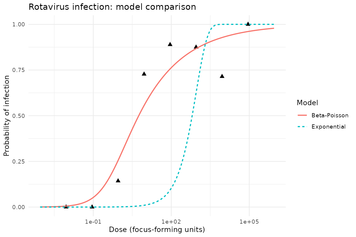
The Ward rotavirus model comparison shows the exponential and beta-Poisson curves with observed infection responses.

Advanced usage

Exact beta-Poisson model (opt-in)

By default the workflow fits the exponential and approximate beta-Poisson models. The exact beta-Poisson model (confluent hypergeometric form, parameterized in alpha/beta) is available as a deliberate opt-in via the models argument. It participates fully in fitting, the N-model comparison, assessment, consensus, and plotting. Because it is roughly an order of magnitude slower to fit, its bootstrap replicate count is controlled separately (exact_bootstrap_times, default 10000; set to zero to fit and compare it without bootstrapping):

analysis <- analyze_dose_response(
  ward,
  models = c("exponential", "beta_poisson", "exact_beta_poisson"),
  bootstrap_times = 10000,       # exponential + approximate beta-Poisson
  exact_bootstrap_times = 10000, # exact beta-Poisson (slower); 0 to skip
  seed = 2026
)

Fitting robustness (multi-start)

When no starting values are supplied, fit_dose_response() fits the model from several candidate starting values and keeps the highest-likelihood result. A single starting value cannot avoid every start-dependent local optimum across the range of real dose-response data — for example an exponential fit to beta-Poisson-shaped data, or a low-infectivity pathogen whose responses appear only at the highest doses. Validated against the QMRA-wiki reference dataset, this multi-start strategy reproduces the CAMRA reference fits far more reliably than a single fixed start. Supplying start explicitly (as the bootstrap warm-start does) uses that value alone, so bootstrap performance is unaffected.

Pooling multiple datasets

When several trials exist for one pathogen, poolability_test() runs the Haas likelihood-ratio test to decide whether they can be combined: it fits each dataset separately and the stacked combination, then compares the deviance difference to a chi-squared distribution (per model). Datasets that pool significantly worse than when fit separately are kept distinct. group_datasets() extends this to find which trials are mutually poolable.

trials <- list(trial_a = data_a, trial_b = data_b, trial_c = data_c)

poolability_test(trials) # are they poolable? (one row per model)
poolability_combinations(trials) # each pair and larger combination, per model
group_datasets(trials)   # which trials group together (per model)

To see which combinations pass or fail, use poolability_combinations(). For three trials it reports A+B, A+C, B+C, and A+B+C. combination identifies the trials, model identifies the fitted model, p_value reports the test result, and poolable is TRUE when the pooled fit does not worsen significantly at the chosen alpha. Inspect converged before trusting a result. The datasets list column retains the exact trial names.

The report includes overlapping combinations; it does not select a final grouping. group_datasets(trials, method = "exhaustive") searches all ways to divide the trials into non-overlapping groups and selects one grouping per model. The default grouping method instead merges compatible groups greedily. Combination reporting and exhaustive grouping both default to at most six trials because their searches grow rapidly. These are exploratory tests without multiple-testing adjustment; passing a test does not prove equivalence. Compare only experiments with matching hosts, units, and endpoints.

Datasets are combined by stacking — each trial's dose groups are kept as separate binomial observations, so repeated doses across trials are preserved (matching the QMRA-wiki pooled-experiment convention), rather than summed.

Try pooling with synthetic data

The bundled pooling-example.csv contains artificial counts for three experiments, A, B, and C, with 100 subjects at each of four doses. A and B have similar curves; C has a much lower response. These are teaching data, not observations from a real pathogen.

path <- system.file("extdata", "pooling-example.csv", package = "singlehit")
raw <- readr::read_csv(path, show_col_types = FALSE)
collection <- list(
  pathogen = "Synthetic example",
  datasets = split(raw, raw$study_id)
)
report <- poolability_combinations(collection$datasets)
report[c("combination", "model", "p_value", "poolable", "converged")]
group_datasets(collection$datasets, method = "exhaustive")

The combination report prints:

# A tibble: 8 × 5
  combination model         p_value poolable converged
  <chr>       <chr>           <dbl> <lgl>    <lgl>
1 A + B       exponential  9.40e- 1 TRUE     TRUE
2 A + B       beta_poisson 9.25e- 1 TRUE     TRUE
3 A + C       exponential  2.50e-66 FALSE    TRUE
4 A + C       beta_poisson 9.60e-62 FALSE    TRUE
5 B + C       exponential  4.06e-67 FALSE    TRUE
6 B + C       beta_poisson 4.31e-62 FALSE    TRUE
7 A + B + C   exponential  5.24e-87 FALSE    TRUE
8 A + B + C   beta_poisson 1.19e-79 FALSE    TRUE

Read the multi-experiment CSV before splitting by study_id. Passing the whole file to read_dose_response() would correctly reject mixed experiment IDs. At alpha = 0.05, A+B passes for both models, while A+C, B+C, and A+B+C fail. All fits converge, and exhaustive grouping puts A and B together with C separate. A and B are candidates for a shared fit; keep C separate. This pooling decision does not establish adequate absolute model fit or create a pooled analysis.

Parallel bootstraps (mirai)

Mirai also works after devtools::load_all(): local workers load the same checkout before starting the bootstrap.

Bootstrap runs above 1,000 replicates automatically use mirai when it is installed and show completion progress while results are collected. If no daemons are already configured, the package starts a temporary pool using 75% of the machine's detected physical cores and removes that pool after collecting the result. Supply workers to override that default:

analysis <- analyze_dose_response(
  ward,
  bootstrap_times = 10000,
  seed = 2026,
  workers = 12
)

Existing mirai daemons are reused and remain under caller control. Use backend = "sequential" to disable automatic parallelization, or configure a pool explicitly:

mirai::daemons(4)
analysis <- analyze_dose_response(ward, bootstrap_times = 10000)
mirai::daemons(0)

Bootstrap samples are generated before parallel dispatch, so the same seed produces identical results with backend = "sequential" and backend = "mirai". Only the model refits are sent to workers.

For a non-blocking bootstrap, start a job and collect it when the result is needed:

fit <- fit_dose_response(ward, "beta_poisson")
job <- bootstrap_dose_response_async(fit, times = 10000, seed = 2026)

# The R console is available while daemons fit the bootstrap samples.
result <- collect_bootstrap(job)

Development

Development notes and owner-requested workflow follow-ups live in TODO.md.

Boosterpak remains optional repository-development tooling. It is not a package dependency and is not needed to install or use singlehit.

For development, the original Ward source file remains at data/raw/Ward_rotavirus.txt. The legacy script is retained under dev/ as a methodological reference; package functions do not source it or depend on its global variables.